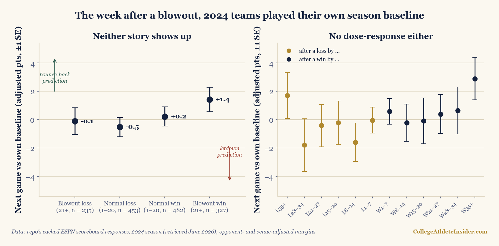
On August 31, Purdue beat Indiana State 49–0. Two weeks later the Boilermakers lost to Notre Dame 66–7 — a 108-point swing between consecutive games, the largest in the cache. Every fan owns a word for each half of that whiplash: the first game set up a letdown, and had the order been reversed, the second would have guaranteed a bounce-back. Both words assert the same testable thing — that last week’s margin, by itself, bends this week’s performance. So I tested both directions at once. Across 1,497 consecutive-game pairs from the 2024 season, teams coming off a blowout win of 21+ points played their next game +1.4 points above their own season baseline (SE 0.9) once the opponent and the venue are accounted for — the wrong sign for a letdown, and statistically nothing. Teams coming off a blowout loss played −0.1 (SE 1.0) — no bounce-back either. The week after a blowout, in both directions, a 2024 team was simply itself. The interesting part is why the myth survives anyway: the unadjusted next-game records — 199–128 after blowout wins, 92–143 after blowout losses — look exactly like momentum, until you notice each group is just matching its own season win rate to the decimal.
What counts here
Same dataset as the margin census and the fourth-quarter audit: my locally cached ESPN scoreboard responses — 877 completed 2024 games, August 24 through December 21 kickoffs (retrieved June 2026), regular season through three of the four CFP first-round games. The cache names 230 teams, but 96 of them are FCS sides appearing once or twice as paid visitors, so the unit of analysis is the 134 teams with eight or more cached games — 1,631 team-games, strung into chronological order per team. A pair is any game followed by another cached game for the same team: 1,497 of them. The trigger is the first game’s result — blowout win (21+, the margin census’s three-score line), normal win, normal loss, blowout loss — and the outcome is the next game’s scoring margin measured against that team’s own baseline: its adjusted margin averaged over its other cached games, with both the trigger game and the next game excluded (10.2 baseline games on average, never fewer than 9). “Adjusted” means two corrections: add the opponent’s season mean margin, and strip a flat home edge of 5.05 points — the cache’s own mean home margin in its 755 FBS-vs-FBS games. Under the null — no memory of last week — every bucket’s deviation should sit at zero.
The census: four buckets, four zeros
| Coming off a … | Pairs | Next W–L | Next win % | Baseline win % | Raw margin dev | Adjusted dev (SE) |
|---|---|---|---|---|---|---|
| Blowout win (21+) | 327 | 199–128 | 60.9% | 60.9% | +0.2 | +1.4 (0.9) |
| Normal win (1–20) | 482 | 266–216 | 55.2% | 56.6% | −1.7 | +0.2 (0.7) |
| Normal loss (1–20) | 453 | 216–237 | 47.7% | 50.8% | −2.0 | −0.5 (0.7) |
| Blowout loss (21+) | 235 | 92–143 | 39.1% | 42.0% | −0.2 | −0.1 (1.0) |
| Any game | 1,497 | 773–724 | 51.6% | 53.5% | −1.2 | +0.2 (0.4) |
Take the letdown first, because it fails most decisively. If a 21-point win breeds complacency, the top row’s adjusted column should be negative. It is +1.4 (SE 0.9) — and the fair test is the contrast against the placebo row below it, teams coming off an ordinary win: +1.2 points, SE 1.1. Zero sits comfortably inside that interval; a letdown worth more than about a point of scoring margin does not. The bounce-back fails identically. Teams humiliated by 21+ came back at −0.1 (SE 1.0) against their own baseline; the contrast against ordinary losers is +0.4, SE 1.2. For scale: a single game’s deviation from a team baseline has a standard deviation around 15 points. These effects, if they exist at all, are one-tenth of one game’s ordinary noise.
Now the illusion. Read the table’s win-rate columns the way a talk show does: teams went 60.9% the week after a blowout win and 39.1% the week after a blowout loss — a 22-point gap that looks exactly like momentum. Then read each row against its own baseline. Teams coming off blowout wins were already 60.9% teams across the rest of their season — agreement to the decimal. Blowout losers were 42.0% teams who went 39.1%. The gap between the rows is not what last week did to this week; it is who gets blown out and who does the blowing out. The same selection runs the repeat rates: a blowout win was followed by another blowout win 26.6% of the time (87 of 327) against a 21.1% base rate — not because the first rout taught anyone anything, but because Indiana kept being Indiana. Ninety-three of the 134 teams logged both a 21+ win and a 21+ loss in the same cached season.
The confound the raw column confesses
The raw column is in the table because it almost sells a false story. Unadjusted, the average next game runs −1.2 points below baseline across all 1,497 pairs — every bucket looks mildly disappointing. That is not psychology; it is scheduling. Openers are bought cupcakes and next-games skew into conference play, so “next week” is systematically harder than “the rest of the season” on average. Opponent adjustment recenters the whole exercise to +0.2 (SE 0.4), which is what a sanity check should read. The season’s biggest “bounce-back,” by swing, is the confound wearing a costume: Western Kentucky lost 0–63 at Alabama on the season’s opening Saturday and won 31–0 the following week — a 94-point recovery achieved by replacing Alabama with Eastern Kentucky. Adjust for the opponents and the miracle evaporates into two ordinary WKU games. Whenever a broadcast cites a team’s record “after a loss,” it is quoting mostly the schedule, the same way the raw column does.
Dose-response is the other knife. If blowouts carry psychological payload, bigger ones should carry more: the 35+ humiliations should out-bounce the 21–27 ones, and the 35+ routs should set up the deepest letdowns. The right panel of the chart shows twelve bands of trigger margin, and no such gradient exists — eleven of the twelve sit within 1.2 SE of zero, in no particular order. The one band that leans anywhere is the wrong direction for the myth: teams coming off wins of 35+ ran +2.9 (SE 1.5) next time out. I read that as residual mismatch, not momentum — 85 of the 327 blowout-win triggers came against sub-8-game (FCS) visitors whose “season margin” is one or two games of data, so the adjustment leans hardest exactly there. Rerun the whole test on FBS-vs-FBS games only and the headline numbers barely move: +1.1 (SE 1.0) after blowout wins, +0.2 (SE 1.0) after blowout losses. Still zeros.
One live lead, flagged as a lead
I cut the pairs one more way — by rest — expecting nothing, and got the article’s only non-zero. Blowouts followed by a normal week (nine days or fewer to the next game, 465 pairs) ran +0.0 (SE 0.7): the headline null, again. Blowouts followed by extra rest — a bye or a long layoff, 97 pairs — ran +4.4 (SE 1.3), and the split is eerily symmetric: +4.6 after blowout wins (n = 47), +4.2 after blowout losses (n = 50). The placebo holds up, too: non-blowout games followed by a bye ran −0.4 (SE 1.0), so this is not a generic rest dividend. Honesty about what this is: a post-hoc cut, found while fishing, in one season, and its gap over the placebo is roughly 2.9 SE before any correction for the several splits I tried. That is a lead for next season’s data, not a finding — if it is real, the story would have to be something like blowouts (played or absorbed) costing less and teaching more than close games, with a bye to bank the difference. File it under “check again with more football.”
And for symmetry, the whiplash census: a 21+ win followed immediately by a 21+ loss happened 27 times (Purdue’s 108-point swing the largest); a 21+ loss followed by a 21+ win, 33 times — Western Kentucky’s 94-point turn from the paragraph above the largest, and the loudest being Indiana falling 38–15 at Ohio State and then winning the Old Oaken Bucket finale 66–0, an 89-point turn by a playoff team against a 1–11 rival. Both lists exist, both make highlight packages, and both are exactly as common as 15-point game-to-game noise says they should be.
Where this can mislead you
- One season, 1,497 pairs. The SEs are the article: the letdown contrast’s 95% interval spans roughly −1.0 to +3.4 points, the bounce-back’s −1.9 to +2.7. Small real effects — a point either way — would hide in there. What the data rejects is the effect the narrative sells, the one big enough to pick games with.
- “Baseline” is a season average. Teams change across a season — injuries, benchings, November weather. A deviation measured against a whole-season baseline treats all of that as noise. It cannot see a letdown that a coach cured by Wednesday.
- The adjustment is two blunt corrections. Opponent season margin and a flat 5.05-point home edge — no schedule-strength iteration, no neutral-site flags, and one-game FCS opponents make their own adjustment nearly circular (the 35+ band’s lean is likely this). The home-field piece shows the true edge varies by slice; I applied one number.
- Sequences have seams. The cache ends December 21, so late-December pairs cross a month of layoff, portal exits, and opt-outs; 300 of the 1,497 pairs have 10+ days between games. The rest split above is exactly where those seams concentrate — another reason to hold it loosely.
- Win rates are unadjusted by construction. The 39.1%-vs-42.0% dip after blowout losses is within noise (SE 3.2 points) and confounded by schedule; the adjusted margin column is the one doing inference.
- Pairs overlap. A 3–9 team contributes consecutive triggers whose baselines share games, so observations are not fully independent; the SEs here treat them as if they were, which makes the intervals, if anything, slightly too narrow — too narrow around zero.
The takeaway
Both halves of the sport’s favorite week-to-week psychology failed the same audit in the same way. After 327 blowout wins, teams played 1.4 points above their baseline — the letdown predicted below, and missed. After 235 blowout losses, they played 0.1 below — the bounce-back predicted above, and missed. No dose-response, no survival under placebo contrast, no change when FCS games are stripped out. What survives instead is selection: blowout winners win next week because they are good, blowout losers lose because they are not, and the 22-point gap between those raw records will keep the myth in business indefinitely because the myth is a real pattern with a wrong caption. The one thread worth pulling — blowout-then-bye at +4.4 — is labelled and shelved until there is more football to test it on. Until then, the honest forecast for any team’s next game, the week after triumph or the week after disgrace, is the least dramatic sentence in sports: they will probably play like themselves. The close-game luck piece reached the same verdict about clutch records; this is the blowout wing of the same building.
Reproduce it
The chart above is rebuilt from the cache on every charts build by charts/chart_letdown_bounce.py, which recomputes every number in this article — the four buckets, the contrasts, the dose-response bands, the rest split, the repeat rates, the named games — and warns if the cache stops reproducing any of them. The core:
adj = lambda r: r.margin + opp_mean[r.opp] - (5.05 if r.home else -5.05)
for team in teams_with_8plus_games:
    for trig, nxt in consecutive_pairs(team):
        base = [g for g in team.games if g not in (trig, nxt)]
        dev = adj(nxt) - mean(adj(b) for b in base)
# blowout wins:  mean dev +1.42 (SE 0.87, n=327)
# blowout losses: mean dev -0.12 (SE 0.95, n=235)
Run python charts/chart_letdown_bounce.py and it prints the full audit before it draws a point.
Sources & further reading
- Theory: Chapter 12: Confidence Intervals: Estimating with Uncertainty — a free chapter at DataField.dev; this whole article is an exercise in reading ±2 SE before reading a narrative.
- Data: my locally cached ESPN public-API scoreboard responses (
scripts/cache/, retrieved June 2026; provenance indata_layer/SOURCE.txt) — 877 completed 2024 games through December 21, finals and venues. - Every figure above is recomputed from that cache at build time by
charts/chart_letdown_bounce.py, which warns if any published number drifts. - Related: the margin census (where the 21+ line and the 29.2% blowout share come from), the fourth-quarter audit (the same cache, inside single games), home-field advantage, measured (why the venue correction exists), and one-score records and luck (the companion myth, audited the same way).