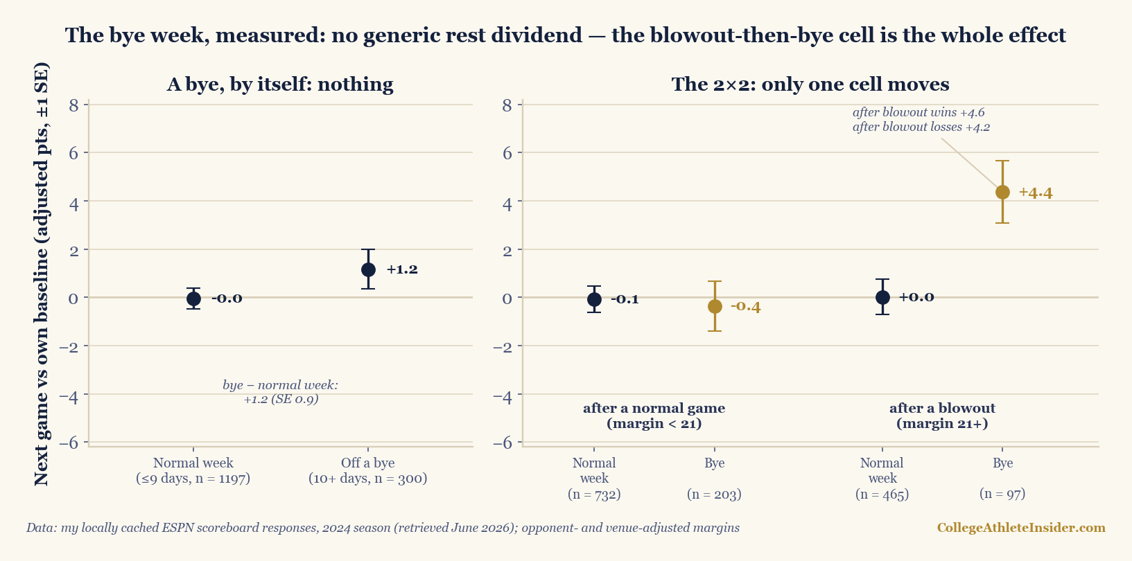
Three days ago, the letdown audit ended with a confession: after finding nothing in either direction of the sport’s favorite momentum myth, I kept one lead I had found while fishing and refused to claim it. Teams coming off a blowout with a bye before their next game ran +4.38 adjusted points above their own season baseline (SE 1.30, n = 97), symmetric across wins (+4.58) and losses (+4.19), while ordinary games followed by a bye ran −0.36 (SE 1.03, n = 203). A post-hoc cut, flagged and shelved. This piece un-shelves it the only honest way available: state that number as the hypothesis before the code runs, declare one primary test, and audit the bye week head-on. Two answers came back. First, the bye itself is worth nothing detectable: all 300 bye-preceded games ran +1.2 points over the 1,197 normal-week games (SE 0.9 on the contrast), a 1.3-SE shrug. Second, the blowout-then-bye cell survived every attempt I made to kill it, and the pre-declared contrast landed at +4.74 points, SE 1.66. The caveat that governs everything: this is the same 877 games the lead crawled out of, so the verdict is consistent with, never confirmed.
The pre-registration, such as it is
Method drift is how follow-ups cheat, so there is none: charts/chart_bye_week.py imports the 8/5 piece’s loader rather than re-implementing it, and every construction choice is carried over verbatim — the same 877 cached 2024 games, the same 134 teams with 8+ cached appearances, the same 1,497 consecutive-game pairs, margins adjusted by opponent season margin and a flat 5.05-point home edge, each next game measured against the team’s own baseline with the trigger and next game excluded. “Bye” keeps the 8/5 definition too: 10+ days between consecutive games. That split is cleaner than the original December-seams caveat feared — 295 of the 300 bye pairs sit between 10 and 16 days (median 14), only 5 are long layoffs. The declared primary test, written down before rerunning anything: blowout-then-bye versus non-blowout-then-bye, one contrast, no shopping. Everything else below is secondary and labelled as such.
A bye, by itself, is nothing
Start with the question the flagged lead skipped past: does rest alone help? Raw, it looks like it hurts — post-bye teams ran −1.6 points below their baselines unadjusted, and went 153–147 (51.0%) against a 53.9% baseline win rate. That is the schedule talking: coaches park byes in front of hard games, and the average post-bye opponent carries a +2.25 season margin versus +0.71 after normal weeks. Adjust for who was actually standing on the other sideline and the bye recovers to +1.17 (SE 0.82), against −0.04 (SE 0.44) for normal weeks — a contrast of +1.21, SE 0.93. That is 1.3 SE: indistinguishable from zero, and small even taken at face value. The bye, by itself, gets the same verdict the letdown and the bounce-back got: not so you could measure it.
The 2×2 the last piece promised
| Cell | Pairs | Adjusted dev (SE) |
|---|---|---|
| Normal game → normal week | 732 | −0.1 (0.5) |
| Normal game → bye | 203 | −0.4 (1.0) |
| Blowout (21+) → normal week | 465 | +0.0 (0.7) |
| Blowout (21+) → bye | 97 | +4.4 (1.3) |
| … after blowout wins | 47 | +4.6 (1.9) |
| … after blowout losses | 50 | +4.2 (1.8) |
The reproduction is exact — +4.38 (SE 1.30, n = 97), +4.58 and +4.19 on the win/loss halves, −0.36 on the placebo — which proves only that the code is deterministic. What the follow-up actually buys is the multiplicity discount, paid up front: on 8/5 this cell was one of several cuts tried while fishing; today it is the single declared test, +4.74, SE 1.66, 2.9 SE from zero — a result that, on independent data, would sit around p ≈ 0.004. The full diff-in-diff across the 2×2, charging the cell for both main effects, is +4.63, SE 1.89. And the shape matters: three cells on zero, one cell four points high, split almost perfectly between teams that had just humiliated someone and teams that had just been humiliated. Whatever this is, it is not “rest helps” and not “revenge motivates.”
Trying to kill it
A 97-pair cell earns a leverage check before it earns a paragraph. The five biggest positive contributors: Arizona off a 24-point loss to Kansas State beating Utah by 13 (+31.7 versus baseline), Memphis off a 35-point UAB rout handling Tulane (+30.4), East Carolina (+28.8), Michigan State (+26.5), Baylor (+26.0). Drop all five: +3.05, SE 1.22 — smaller, still 2.5 SE from zero. That test is rigged against any positive mean; the same deletion drags the placebo to −1.15. The fair version trims both tails, five and five: +4.51, SE 1.09 — essentially the headline. Strip every game touching an FCS opponent, where the adjustment is weakest: +3.95 (SE 1.39, n = 87) against a placebo of −0.85 (SE 1.05). The 97 pairs come from 75 different teams, none contributing more than 3 (Navy). And the heterogeneity probes stayed boring in the right way — post-bye favorites (by season margin) +5.19 (SE 1.76, n = 40) versus underdogs +3.81 (SE 1.84, n = 57); byes ending by October 31 +4.70 (SE 1.72, n = 55) versus later +3.96 (SE 1.99, n = 42). No subgroup carries the effect; none contradicts it. If this were three outliers in a trench coat, one of these knives finds the seam. None did.
The wins problem
Here is the deflation the effect earns anyway: four points of margin bought almost no wins. Blowout-then-bye teams went 49–48 against a 49.8% baseline expectation — and the blowout losers, the +4.2-margin half, went 18–32, because playing four points over a bad baseline still loses, and the post-bye schedule is cruel. Alabama is the poster child and the counterexample in one season: off a 34-point demolition of Missouri and a bye, the Tide beat LSU by 29 (+23.3 versus baseline); off a 32-point demolition of Wisconsin and a bye, they edged Georgia by 7, a dead-ordinary −4.2. A four-point mean under a 15-point game-to-game standard deviation moves betting margins, not standings, and anyone reading this as “blowout + bye = lock” has left the data behind.
Where this can mislead you
- Same season, same games — the big one. The hypothesis was born in this exact cache, so reproducing it here is arithmetic, not evidence. The follow-up pays the multiplicity bill; it cannot buy independence. “Consistent with” is the ceiling until this exact test reruns on a cached 2025 season.
- n = 97. The cell’s 95% interval spans roughly +1.8 to +7.0 points — wide enough to hold a modest curiosity and a headline at once.
- Byes are assigned in the preseason. That cuts both ways: a blowout landing just before a scheduled bye is close to random (good for causal reading), but bye placement itself is not random across the calendar, and the opponent had two weeks to prepare for you too.
- The adjustment is the 8/5 piece’s, bluntness included — opponent season margin plus a flat 5.05-point home edge, near-circular for FCS opponents. The FBS-only rerun is the mitigation, not a cure.
- Five pairs are long layoffs, not byes (17+ days); removing them moves the blowout-bye cell from +4.38 to +4.26. Negligible.
- Pairs overlap and SEs assume independence, same as 8/5 — the intervals are, if anything, slightly too narrow.
The takeaway
The generic bye week — the one broadcast crews credit for every post-idle upset — measured +1.2 points and 1.3 SE in 2024: nothing, and even the “post-bye teams struggle” counter-myth is just tougher scheduled opponents wearing a narrative. The specific thing the letdown piece flagged — a blowout, in either direction, followed by two weeks to digest it — came back +4.4 points, 2.9 SE over its placebo as a single pre-declared test, and shrugged off every audit this dataset can host. That is as far as one season of data can carry a claim, and I am stopping exactly there. If the mechanism is real — blowouts costing less and teaching more than close games, with a bye to bank the lesson — it will still be there in the 2025 cache, where the test is already written and no fishing is required. That rerun, not this reproduction, is the verdict. Until then the bye week stays what the numbers say it is: two weeks of nothing, except — maybe — after a massacre.
Reproduce it
The chart above is rebuilt from the cache on every charts build by charts/chart_bye_week.py, which imports the 8/5 module’s loader (so the two pieces cannot drift apart), recomputes every number in this article — the main effect, the 2×2, the declared contrast, the leverage trims, the FBS-only rerun, the heterogeneity probes, the named games — and warns if the cache stops reproducing any of them. The core:
bye   = pairs(any_game, min_gap=10)        # n=300: +1.17 (SE 0.82)
short = pairs(any_game, max_gap=9)         # n=1197: -0.04 (SE 0.44)
# declared primary test, stated before rerunning:
blow_bye    = pairs(blowout, min_gap=10)   # n=97:  +4.38 (SE 1.30)
placebo_bye = pairs(normal,  min_gap=10)   # n=203: -0.36 (SE 1.03)
# contrast: +4.74 (SE 1.66); diff-in-diff: +4.63 (SE 1.89)
Run python charts/chart_bye_week.py and it prints the full audit before it draws a point.
Sources & further reading
- Theory: Chapter 16: Comparing Two Groups — a free chapter at DataField.dev; this article is one declared two-group contrast plus the discipline of not running twenty.
- Data: my locally cached ESPN public-API scoreboard responses (
scripts/cache/, retrieved June 2026; provenance indata_layer/SOURCE.txt) — 877 completed 2024 games through December 21, finals and venues. - Every figure above is recomputed from that cache at build time by
charts/chart_bye_week.py, which warns if any published number drifts. - Related: the letdown and the bounce-back (the piece that flagged this lead and set the method), the margin census (the 21+ blowout line), home-field advantage, measured (the venue correction), and one-score records and luck (what margins say that win-loss records cannot).