From Point Spread to Win Probability: The Math of a College Football Favorite

“They’re favored by a touchdown.” You hear it every Saturday, and most fans file it under they should win without ever asking how often. Here is the useful part up front: a point spread is not a vibe, it is the market’s estimate of the expected final margin, and if you are willing to grant one assumption — that real margins scatter around that estimate like a bell curve — the spread converts to a precise win probability. A seven-point college favorite comes out to about 67%. Not “should win.” Wins two times in three, loses the other time. My whole argument here is that people badly overrate single-digit favorites, and the math says so cleanly.

Let me be honest about what this is before we go further: this is a clearly-labeled model, not game data. I did not pull a database of finals and count. The numbers below come from the normal win-probability model — the same family of model-based pieces I’ve been writing lately. That’s a legitimate way to think, but it leans on one assumption (the spread of the bell), and I’ll keep flagging that so you never mistake an illustration for a measurement.

The one idea: the spread is the center of a bell

Picture the final margin as a dart thrown at the spread. The market says the favorite should win by, say, 7. Reality rarely lands exactly there — sometimes the favorite wins by 21, sometimes the underdog pulls the upset. If those outcomes pile up symmetrically around 7 in the shape of a normal bell, then the favorite wins whenever the dart lands to the right of zero (a margin above zero means the favorite covered the win, not the spread). The probability of that is simply the area of the bell to the right of zero. Written out:

P(favorite wins) = Φ(spread / σ)

where Φ is the standard normal CDF — the cumulative area under the bell — and σ (sigma) is the standard deviation of the final margin around the spread. That single division, spread divided by sigma, turns a number of points into a number of standard deviations, and Φ turns standard deviations into a probability. That’s the entire model.

What sigma should be for college football

Sigma is the whole ballgame, so it deserves a real answer. College football margins scatter more than the NFL’s — more plays per game, more possessions, more scoring, and far bigger blowouts when a top-15 team hosts a tune-up. The well-known result from the spread literature is that NFL final-margin standard deviation sits around 13.5 points. College runs wider; about 16 points is a reasonable FBS value, and I’ll treat that as the central estimate. To keep myself honest I’ll show a band of σ = 14 and σ = 18 around it.

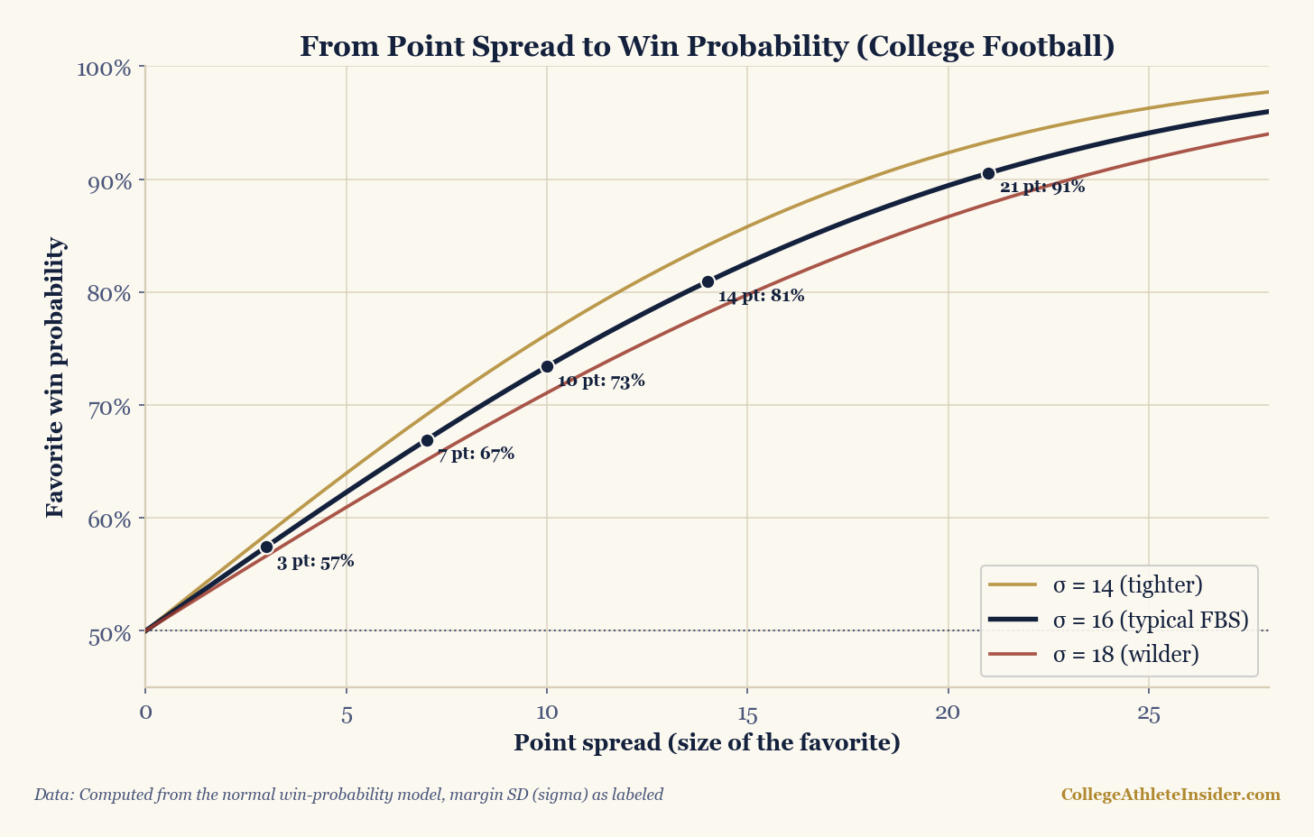
Read the middle curve and the headline finding jumps out: single-digit favorites are not safe. At σ = 16, a 3-point favorite wins just 57.4% of the time — barely better than a coin flip. A 7-point (touchdown) favorite is 66.9%, meaning it loses outright a full third of the time. You have to climb to a 10-point favorite (73.4%) before it feels comfortable, a 14-point two-touchdown favorite (80.9%) before it’s genuinely lopsided, and a 21-point favorite (90.5%) before you can start treating a loss as a real shock. The fan who says a touchdown favorite “should win” is right — but “should win two-thirds of the time” is a very different sentence than the one most people are actually thinking.

Work one out, end to end

Take the touchdown favorite and run it all the way to a betting number. Spread is 7, sigma is 16:

• Convert points to standard deviations: z = spread / σ = 7 / 16 = 0.44.
• Look up the normal CDF: Φ(0.44) ≈ 0.669. (That’s the area of the bell to the left of 0.44 standard deviations above the mean.)
• So P(favorite wins) ≈ 66.9%, call it 67%.

Now make it concrete by converting to fair moneyline odds, no juice. A favorite’s fair American price is −100 × p / (1 − p). Plug in 0.669: −100 × 0.669 / 0.331 ≈ −203. So a touchdown favorite, under this model, is a fair −203 on the moneyline — you’d risk about $203 to win $100. If a book is hanging that same team at −260, the model thinks the favorite is overpriced and the underdog is the value. That’s the payoff of the conversion: one fuzzy phrase became a probability and then a price you can shop against.

How little sigma actually matters here

Sigma is an assumption, so the fair question is: how much does my answer wobble if I guessed it wrong? Less than you’d fear. Hold the touchdown favorite and slide sigma across the band: σ = 14 gives 69.1%, σ = 18 gives 65.1%. The center case was 66.9%. So whether I’m a little too tight or a little too loose on the spread of outcomes, a touchdown favorite is “roughly two in three” either way. That robustness is exactly why I trust the qualitative claim — single-digit favorites are overrated — even while admitting I don’t know sigma to the decimal.

One more structural fact worth carrying around: near a pick’em, each additional point of spread is worth about 2.5 percentage points of win probability. That’s the slope of the curve at zero. The curve is steepest in the middle and flattens toward the extremes — the move from 0 to 3 points buys you far more probability than the move from 18 to 21. It’s the same reason a key field goal in a tied game swings things harder than the same field goal in a blowout, which is the through-line in when is a lead safe.

Where this model lies to you

I like this tool, but only because I know its seams:

• Sigma is assumed, not measured here. I picked 16 from the literature; I did not fit it to a dataset in this piece. And sigma isn’t even constant — it widens for high-total shootouts where both offenses are humming, and shrinks for defensive slugfests where everyone’s grinding out field goals. A single sigma is a convenient fiction.
• The normal model ignores college football’s key numbers. Real margins are not perfectly smooth; they clump on 3 and 7 because of how scoring works — one possession, one score. A smooth bell can’t see that clustering, so it slightly misprices spreads sitting exactly on 3 or 7. The saving grace is that this clustering is weaker in college than in the NFL, precisely because CFB margins are more spread out, so the normal approximation actually fits college better than it fits the pros.
• The spread itself can be wrong. Φ(spread / sigma) inherits whatever bias is baked into the spread. A stale line that hasn’t absorbed a quarterback injury feeds a confidently wrong probability. The model can only be as good as its center.
• A model is only as good as sigma. Garbage in, garbage out — everything above hangs on that one parameter.

If you want the bigger picture on how these probabilities get built and stress-tested, I walk through the machinery in win-probability models for college football. And because this whole post assumes regulation can end in a clean margin, it’s worth remembering the tail where it doesn’t: how college football overtime math works changes the shape of close finishes in ways the bell ignores. The quality of the spread you feed in, meanwhile, is downstream of strength of schedule — a rating that hasn’t adjusted for who a team has played will hand you a biased center.

The roots, and how to reproduce it

None of this is original to me. Turning a margin into a probability with a z-score and the normal CDF is the approach Wayne Winston lays out in Mathletics, and the “NFL margin SD is about 13.5” figure is a staple of the Pythagorean and spread literature; college simply runs wider. The reproducibility is the appealing part: there are no hidden coefficients. It is literally Φ(spread / sigma) with Φ the standard normal CDF. Every number in this article is recomputed by charts/chart_spread_to_winprob.py, which evaluates that one expression across spreads from 0 to 21 at sigma values of 14, 16, and 18. If you want to feel the curve in your hands — or run Elo ratings into spreads of your own — the win-probability tools on the calculators page do exactly this conversion live.

So the next time someone shrugs that their team is “favored by a touchdown,” you can tell them the truth: that’s a 67% team, a fair −203, and a one-in-three chance of going home unhappy. Single-digit favorites are coin flips wearing a confident jersey.