Not every analysis needs Python. A pivot table — the most underrated feature in any spreadsheet — can summarize a whole college football season by team, conference, month or situation in about a minute, no formulas required. The trouble with most pivot-table tutorials is that they demonstrate on invented sales data, so you never find out what the tool is like on a real, messy season file. This one uses the season file this site actually publishes from: 877 completed 2024 college football games out of my locally cached ESPN scoreboard responses. Every table below is a pivot I built from those rows, and every number in them is recomputed from the cache at build time by charts/chart_pivot_conference_margin.py, which warns if the data stops reproducing what is printed here.
The file we are pivoting
The dataset is the same one behind the margin-distribution piece and the overtime census: 877 completed games, August 24 through December 21 kickoffs (retrieved June 2026) — the regular season, the conference championships, Army–Navy, and three of the four CFP first-round games. The quarterfinals onward and the January bowls are not in the cache, so nothing here speaks to them.
Flattened into a sheet, one row per game, it looks like this:
| Date | Home | HomePts | Away | AwayPts | Margin | Conference | ConfGame |
|---|---|---|---|---|---|---|---|
| 2024-10-05 | … | … | … | … | … | SEC | TRUE |
| 2024-10-05 | … | … | … | … | … | Big Ten | TRUE |
| 2024-09-07 | … | … | … | … | … | ACC | FALSE |
| 2024-11-30 | … | … | … | … | … | MAC | TRUE |
Two of those columns are not scores and are worth a sentence each, because they are what makes the pivots below mean anything. Conference is the feed's own groups.shortName for the game — I do not hand-type a membership list anywhere, which matters in a realignment era when any list I typed would be wrong within a year. ConfGame is the feed's conferenceCompetition flag: it is true for 528 of the 877 games and false for the other 349. Conference championship games are not flagged, so they sit in the non-conference pile; that is the feed's convention and I keep it rather than patching it, so the number is reproducible by anyone reading the same responses.
Add one helper column while you are here: Margin = ABS(HomePts - AwayPts). Absolute value, deliberately — a pivot on signed home margin measures home-field advantage, which is its own article and its own set of traps. Everything below is about how lopsided games were, not who won them.
If you want to build this file yourself, my CSV pipeline tutorial writes exactly this shape out of the same public endpoint. Open the CSV in Excel or Google Sheets and you are ready.
Step 1: insert the pivot
- Excel: select the data → Insert → PivotTable.
- Google Sheets: select the data → Insert → Pivot table.
You get an empty pivot with four drop zones: Rows, Columns, Values, and Filters. Everything that follows is dragging fields into those four zones. No formula is written after this point.
Step 2: Rows = Conference, Values = Margin
Filter to ConfGame = TRUE, drop Conference into Rows, and drop Margin into Values four times: once as Count, once as Average, once as Median (Excel needs a MEDIAN measure or Power Pivot for this; Sheets offers it in the summarize menu), and twice more as counts you will convert to rates in step 4. Sort by average descending. That is the whole build, and here is what the 2024 conference schedule says:
| Conference | Games | Avg margin | Median | One-score (1–8) | Blowout (25+) |
|---|---|---|---|---|---|
| Big Ten | 81 | 17.2 | 15 | 38.3% | 25.9% |
| Big 12 | 72 | 14.0 | 10 | 43.1% | 19.4% |
| ACC | 68 | 12.1 | 9 | 50.0% | 16.2% |
| SEC | 64 | 14.0 | 12 | 34.4% | 15.6% |
| Sun Belt | 56 | 14.8 | 13 | 39.3% | 17.9% |
| American | 56 | 19.7 | 17 | 26.8% | 33.9% |
| MAC | 48 | 14.2 | 11 | 37.5% | 18.8% |
| Mountain West | 42 | 12.9 | 10 | 47.6% | 9.5% |
| C-USA | 40 | 13.3 | 9.5 | 45.0% | 15.0% |
One drag, and “which league plays the closest games” stops being an argument and becomes a table. The ACC played the tightest conference schedule in the cache: an average margin of 12.1, a median of 9, and exactly half its 68 league games decided by one score. The American played the most lopsided: 19.7 average, a third of its games decided by 25 or more. The Big Ten played 81 conference games, more than any other league in the cache, and posted the second-highest blowout rate of the nine at 25.9%. Depth and competitiveness are not the same measurement, and the pivot separates them in about a minute.
Two housekeeping notes the pivot will show you and the prose should not hide. The Pac-12 appears in the row list with one cached 2024 conference game, decided by 3 points; a single-game row is a label, not a measurement, so I leave it out of the table above rather than let it sort to the top. And the count column is not decoration — it is the column that tells you which rows you are allowed to read.
Step 3: add a Column field — margin by conference and month
A pivot becomes a cross-tab the moment you drag a second field into Columns. Put the month of Date there, keep Conference in Rows and average Margin in Values, and the one-dimensional table above turns into a grid:
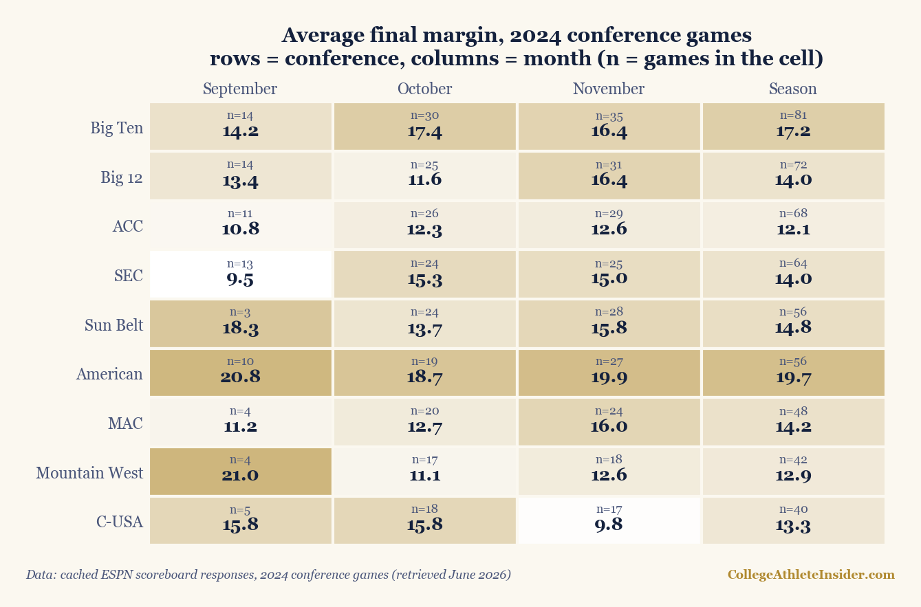
charts/chart_pivot_conference_margin.py.The grid pays for itself immediately. The SEC's season average of 14.0 is a blend of a genuinely tight September (9.5 across 13 games, the lowest single cell in the grid) and a much rougher October and November (15.3 and 15.0). C-USA runs the other way: 15.8 in both September and October, then 9.8 in November, its 17 late games the tightest November cell in the grid. Neither pattern is visible in the season column, and neither took a formula to find.
It is also where you meet the pivot table's favorite failure mode. The Sun Belt's September cell reads 18.3 — on three games. Mountain West September reads 21.0 on four. Those cells are noise wearing a decimal point, which is exactly why the count belongs in the grid next to the average. A pivot will compute a mean of one row as happily as a mean of a thousand, and it will not tell you which one you are looking at.
Step 4: “Show values as % of row total”
The single most useful setting in the Values zone turns counts into rates without a formula. Bucket Margin into the four bands this site uses — 1–8, 9–16, 17–24, 25+ — put the month in Rows and the band in Columns, drop Margin into Values as a Count, then choose Show values as → % of row total (Excel) or Show as → % of row (Sheets). Across all 877 cached games:
| Month | Games | 1–8 | 9–16 | 17–24 | 25+ | Conference games |
|---|---|---|---|---|---|---|
| August | 85 | 17.6% | 11.8% | 22.4% | 48.2% | 1 |
| September | 275 | 32.0% | 11.6% | 20.7% | 35.6% | 78 |
| October | 223 | 40.4% | 23.8% | 14.8% | 21.1% | 203 |
| November | 268 | 39.6% | 20.1% | 17.2% | 23.1% | 235 |
| December | 26 | 26.9% | 19.2% | 23.1% | 30.8% | 11 |
Read down the 25+ column and the season has a shape: 48.2% of August games were decided by 25 or more, against 21.1% in October. Read the last column and the shape has an explanation. August is 1 conference game out of 85; October is 203 out of 223. The sport does not become more competitive as the leaves turn — the schedule stops selling guarantee games and starts making teams play their own conference. The same contrast falls straight out of the ConfGame filter: the 528 conference games averaged a 14.8-point margin, the 349 non-conference games 24.1.
The average-of-averages trap, with the actual numbers
Every pivot-table warning list mentions this one and almost none of them show it costing anything, so here it is costing something. The five monthly average margins in the table above are 28.5, 20.8, 14.6, 16.1 and 19.2. Average those five numbers and you get 19.8. The average margin over all 877 games is 18.5. The gap is 1.3 points, and it is entirely August's doing: 85 games carrying the same weight in the second calculation as October's 223.
The fix is not clever, it is structural: aggregate from the raw rows, never from a summary. In pivot terms, put Margin into Values as an Average over the whole dataset and let the pivot re-scan the rows, rather than averaging a column of cells that a previous pivot produced. If you find yourself building a pivot on top of a pivot's output, that is the moment to stop and go back to the source rows.
Filters, slicers, and when to leave the spreadsheet
Drag Conference or ConfGame or a date range into the Filters zone and every table above re-scopes at once; in Excel, Insert → Slicer gives you clickable buttons for the same thing and turns a static sheet into a small dashboard. This is what pivots are genuinely best at: finding the question. Twenty seconds of dragging produced three findings above that I would otherwise have had to guess were worth a script.
The moment to switch to code is when you need the answer to be reproducible. A pivot lives in a file and remembers nothing about how it was built; the version of these tables that this site publishes is regenerated from the cache on every build and audited against the printed figures. That is also the honest limit of everything above: it is one cached season, the conference labels are the feed's, championship games sit outside the 528 by the feed's convention, and nothing here has been adjusted for who played whom. A pivot table measures the schedule as much as the sport — the August column is proof.
Reproduce it
The Python equivalent of the step-2 pivot is one groupby. This is the core of what the build-time script runs, and it prints the full audit before it draws anything:
conf = [g for g in games if g["conf"]]                 # 528 of 877
for name in ["Big Ten", "Big 12", "ACC", "SEC", "Sun Belt",
             "American", "MAC", "Mountain West", "CUSA"]:
    ms = [g["margin"] for g in conf if g["grp"] == name]
    print(name, len(ms), round(sum(ms) / len(ms), 1),
          round(100.0 * sum(1 for m in ms if m <= 8) / len(ms), 1))
# -> Big Ten 81 17.2 38.3 | ACC 68 12.1 50.0 | American 56 19.7 26.8groupby with a GUI. Learn either and the other reads itself.
Run python charts/chart_pivot_conference_margin.py and it recomputes every figure on this page against the cache, warns on any that stops reproducing, and rebuilds the grid image above.
Sources & further reading
- Data: my locally cached ESPN public-API scoreboard responses (
scripts/cache/, retrieved June 2026; provenance indata_layer/SOURCE.txt) — 877 completed 2024 games, August 24 through December 21, of which 528 carry the feed'sconferenceCompetitionflag. - Recomputation and chart:
charts/chart_pivot_conference_margin.pyin this site's build repository, which pins every number above and warns on drift. - See also Chapter 9: Reshaping and Transforming Data (DataField.dev).
- Microsoft: Create a PivotTable to analyze worksheet data · Google: Create and use pivot tables
- Related: Export tidy CSVs with pandas · Build a ranking in a spreadsheet · The same season, banded by margin